Density matrix: distinguishing pure and mixed states
In quantum mechanics, a density operator is a tool for representing completely a two-level quantum system, like a qubit: a density matrix is the representation of a density operator. This formalism can be extended to multi-qubit systems, but it is out our interest here.
In this article, we are going to talk about density matrices as tools for representing quantum states with more generality than quantum kets, we will outline the main properties of these tools and show how they can be used to represent both pure states and mixed states in quantum mechanics. Finally we will see how everything works in a practical example.
density matrix
Article contents
Definition
From the definition provided, four properties can be verified for a density operator, namely \begin{align} I)& \hspace{0.5cm} \hat{\rho}^2 = \hat{\rho} \hspace{1cm} \text{$\hat{\rho}$ is a projector}\\ II)& \hspace{0.5cm} \hat{\rho}^{\dagger} = \hat{\rho} \hspace{1cm} \text{$\hat{\rho}$ is Hermitian}\\ III)& \hspace{0.5cm} Tr(\hat{\rho}) = 1 \hspace{1cm} \text{Normalization}\\ IV)& \hspace{0.5cm} \hat{\rho} ≥ 0\hspace{1cm} \text{$\hat{\rho}$ is positive semidefinite} \end{align}
Let’s proceed to prove these properties form the definition provided above. Properties I and II are obvious from the definition. Let’s prove property III
the density operator formalism also lets use compute expectation values of operators on the quantum state.
We have seen how the density operator formulation provides a legitimate way of representing quantum pure state satisfying their quantum mechanical properties while providing a way of computing expectation values easily. The main reason we use density matrices, however, is that it allows us to describe, with the same tools, pure states and mixed states: let’s define what is the difference between pure and mixed states and then show how density operators can easily represent both.
Pure states and mixed states
On the other hand, a mixed state is a state which can't be described with a ket $|\psi\rangle$, but rather by a probabilistic ensamble of pure states $\{p_i, |\psi\rangle_i\}_{i = 1, ..., N}$.
Let's see how these two kinds of states behave differently when measuring some observable over them.
Given a pure state, if we measure the expectation value of some operator $\hat{O}$ over it, in general the result will be a random variable, only due to the probabilistic nature of quantum mechanics.
When measuring the expactation value of some operator on a mixed state, we have two different sources of randomness, namely the probabilistic nature of quantum mechanics (for each pure state in the ensemble) and the probablistic nature of the ensemble itself. We can refer to the first one as quantum randomness and to the second one as classical randomness. We can picure this "double randomness" in the following way: when measuring an observable on a mixed state, first one of the pure states of the ensamble is selected randomly (classical randomness) and then a quantum measurement is done on this pure state, having a random outcome (quantum randomness).
This also means that a pure state is a state for which we have the maximum possible information, a mixed states on the other hand has an additional source of randomness and we have less information about it.
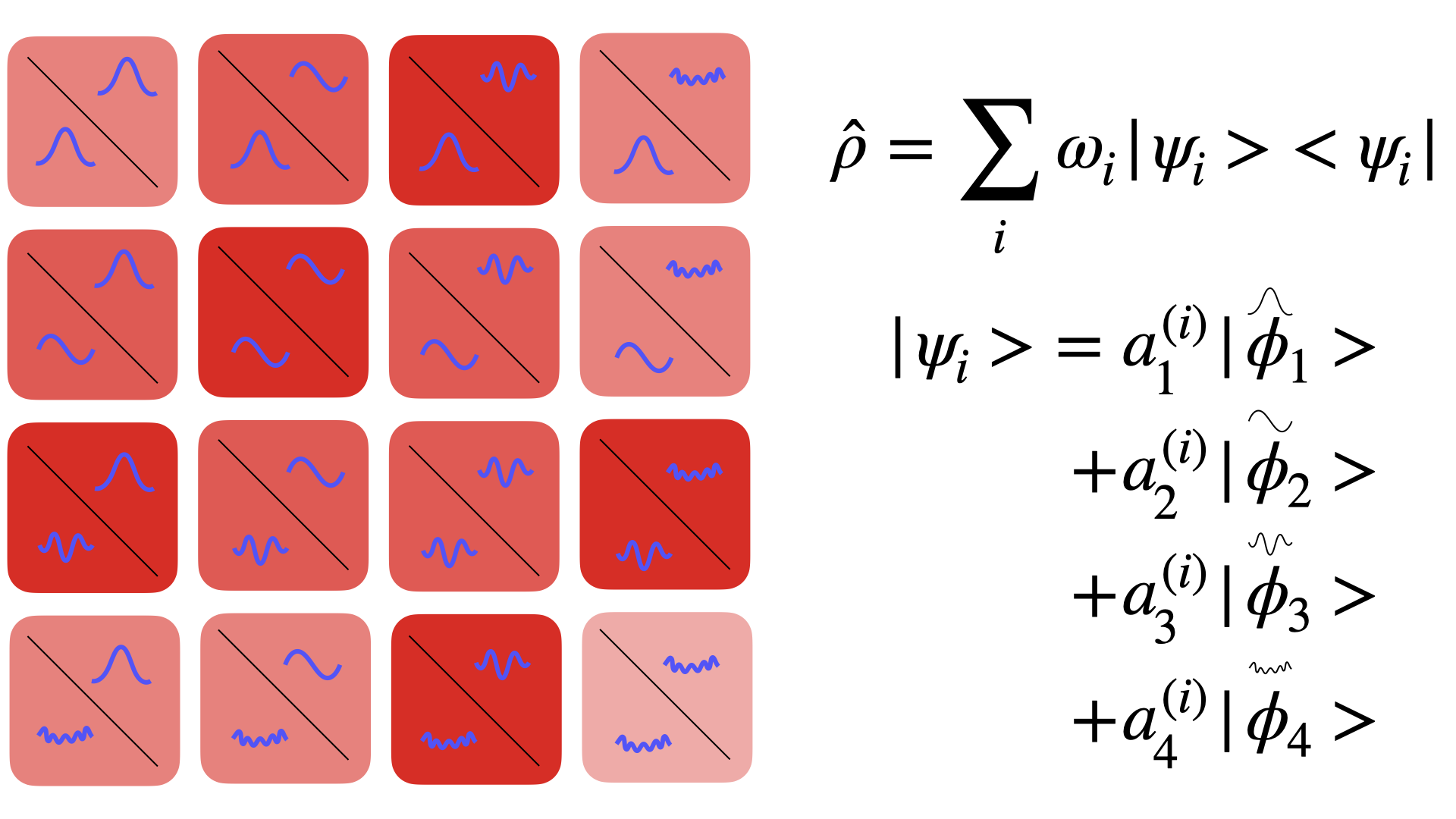
It turns out that density operators can be used to represent both pure states and mixed states and therefore provide a more poweful tool than kets for representing quantum states. We already know how to write the density operator for a pure state
However property I doesn't hold, in fact \begin{equation} \hat{\rho}^2 = \sum_{ij} p_i p_j |\psi_i\rangle \langle \psi_i|\psi_j\rangle \langle \psi_j| = \sum_{ij} p_i p_j |\psi_i\rangle \delta_{ij} \langle \psi_j| = \sum_i p^2_i |\psi_i\rangle \langle \psi_i| \neq \hat{\rho} \end{equation} this gives us a simple way of identifying mixed states from pure states in the density operator formalism, namely by checking whether or not $\hat{\rho}^2 = \hat{\rho}$.
Example
Let’s now provide a example to outline the difference between pure states and quantum states using density operators. Suppose we have an apparatus A producing multiple copies of the following pure state
we see that the off diagonal terms are the ones making the difference between the two density operators. Let’s now see how they behave differently when measuring an observable.
In both cases, we obtain the states $|0\rangle$ and $|1\rangle$ with $50\%$ probability and there is no way of distinguishing between the two states in this experimet. What happens if we measure in the rotated basis $\{|+\rangle, |-\rangle\}$?
The apparatus A produces $\lvert +\rangle$ states, therefore we will get the same outcome for every copy of the system. The apparatus B produces the state $|0\rangle$ and $|1\rangle$ with $50\%$ probabilities. We can rewrite these two states as \begin{equation} |0\rangle = \frac{|+\rangle + |-\rangle}{2} \end{equation} \begin{equation} |1\rangle = \frac{|+\rangle - |-\rangle}{2} \end{equation} therefore the outcome will be in both cases $|+\rangle$ $50\%$ of the times and $|-\rangle$ $50\%$ of the times. We have seen that measuring in a different basis makes us appreciate the difference between $\hat{\rho}^{(A)}$ and $\hat{\rho}^{(B)}$.
Let's now try to compute the expectation values of $\hat{\rho}^{(A)}$ and $\hat{\rho}^{(B)}$ on two operators to make some practice with the formulas explained above: let's chose $\hat{\sigma}_x$ and $\hat{\sigma}_z$. We have \begin{equation} \langle \hat{\sigma}_x\rangle_{\hat{\rho}^{(A)}} = Tr\Big[ \frac{1}{2}\begin{pmatrix} 1 & 1 \\ 1 & 1 \end{pmatrix} \begin{pmatrix} 0 & 1 \\ 1 & 0 \end{pmatrix} \Big] = \frac{1}{2} Tr \begin{pmatrix} 1 & 1 \\ 1 & 1 \end{pmatrix} = 1 \end{equation} \begin{equation} \langle \hat{\sigma}_x\rangle_{\hat{\rho}^{(B)}} = Tr\Big[ \frac{1}{2}\begin{pmatrix} 1 & 0 \\ 0 & 1 \end{pmatrix} \begin{pmatrix} 0 & 1 \\ 1 & 0 \end{pmatrix} \Big] = \frac{1}{2} Tr \begin{pmatrix} 0 & 1 \\ 1 & 0 \end{pmatrix} = 0 \end{equation} \begin{equation} \langle \hat{\sigma}_z\rangle_{\hat{\rho}^{(A)}} = Tr\Big[\frac{1}{2} \begin{pmatrix} 1 & 1 \\ 1 & 1 \end{pmatrix} \begin{pmatrix} 1 & 0 \\ 0 & -1 \end{pmatrix} \Big] = \frac{1}{2}Tr\begin{pmatrix} 1 & 1 \\ -1 & -1 \end{pmatrix} = 0 \end{equation} \begin{equation} \langle \hat{\sigma}_z\rangle_{\hat{\rho}^{(B)}} = Tr\Big[ \frac{1}{2} \begin{pmatrix} 1 & 0 \\ 0 & 1 \end{pmatrix} \begin{pmatrix} 1 & 0 \\ 0 & -1 \end{pmatrix} \Big] = \frac{1}{2} Tr \begin{pmatrix} 1 & 0 \\ 0 & -1 \end{pmatrix} = 0 \end{equation}
also in this case measuring the expectation value on different operators lets us appreciate the difference between a pure and mixed state.
Bibliography
[1] Nielsen, M.A. and Chuang, I., 2002. Quantum computation and quantum information.