The intuition behind kernel methods
With kernel methods we refer to a set of algorithms used in machine learning to perform typically non-linear classification tasks using a similarity measure called kernel. In this article we will see how this similarity measure can be written as a scalar product into a higher dimensional space through a feature map and provide an example of kernel method, namely a kernelized support vector machine (KSVM).
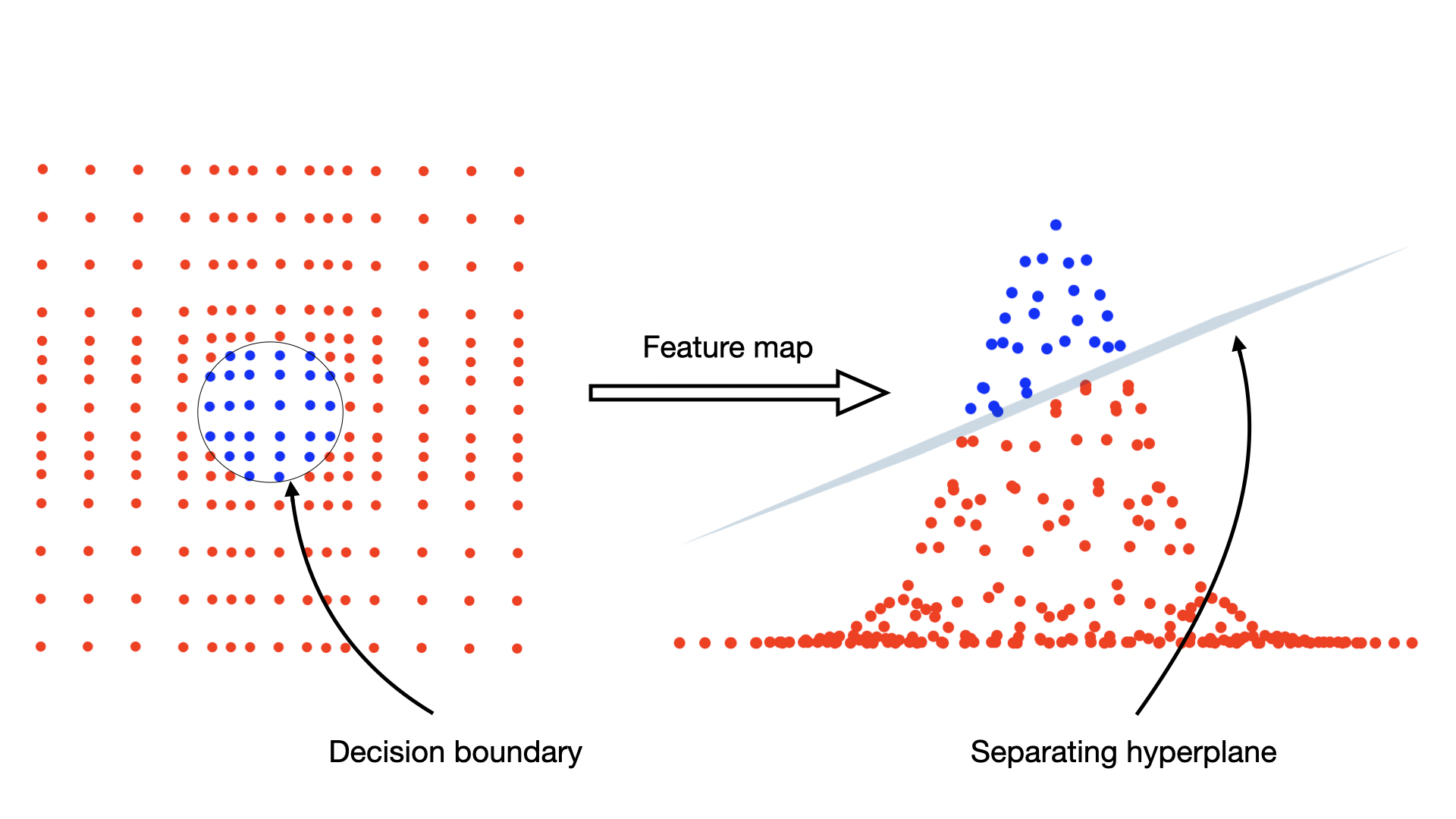
Kernelized SVM method visualized
Introduction
Kernel methods rely on the definition of kernel, namely a similarity function that lets us perform non-linear classification tasks by expressing them as linear problems in higher dimensional spaces. Let’s take a dataset
Let's also define a feature map \begin{equation} \Phi: \mathcal{X} \longrightarrow \mathcal{H} \end{equation} where $\mathcal{H}$ is a higher dimensional space referred to as feature space. A kernel $k: \mathcal{X} \times \mathcal{X} \longrightarrow \mathcal{R}$ is defined as \begin{equation} k(x, y) = \langle\Phi(x), \Phi(y)\rangle \end{equation} in other words a kernel is the scalar product between two data points once they have been mapped to the feature space through the feature map $\Phi$. The advantage of such a scheme, is that it allows us to work in a dot product space where efficient algorithms as SVMs can be exploited.
Thought the formal definition already says it all, it's very difficult to have a feeling of why we define kernels this way and how they can really be used: to fix this, let's start with a practical example
Support vector machine
Let’s start by investigating a common linear classification algorithm in machine learning, namely support vector machines (SVM). This is one of the most common cases in which kernels can be used to improve a linear algorithm giving it non-linear capabilities.

A simple 2D dataset
Distinguishing the two pieces of the dataset optimally (an linearly) means finding an hyperplane which provides a separation between the two classes with the maximum possible margin, where the margin is defined as the smallest distance between the hyperplane and the data points. Let’s look at the following figure

Optimal and non optimal margin (respectively in yellow and green)
in the figure above we can see an example of an optimal margin (yellow) which maximizes the separation between the two classes. On the other hand the second hyperplane (green) still separates the two datasets but with a smaller margin: the first one is the one we are looking for. How can we characterize this hyperplane?

Support vector machine details
This kind of optimization problem is also known as a constrained optimization problem and can be solved by the Lagrangian multipler method.
Kernelized support vector machine
Let’s now introduce kernels and see how they can be used to extend SVMs to non-linear classification problems showing this way one of the most common applications of this idea. Let’s look at a different dataset like the one in the figure below

Dataset non-linearly labeled
the red and blue color identify again two different labels and the goal is to find a rule to separate between these two data points, this rule is evident to the “human eye”, not so much for a classification algorithm. There is clearly no linear rule that lets us do this separation without making huge errors, therefore the SVM approach we just discussed turns out to be useless, but is there a way to somehow manipulate this dataset making it “solvable” by a SVM? Of course yes, this is where the idea of kernels comes into play: we can map these points from a 2D space to a higher dimensional space with some map (called a feature map) and try to see if the dataset is linearly separable in this higher dimensional space, let’s try the feature map mapping from 2D to 3D
this produces the following dataset, which now lives in a three-dimensional space

Projection of the dataset in the feature space
the points have been extruded by the effect of the feature map whe chose and they are now much easier to separate by a linear classifier, namely a plane

Data classifier in the feature space
therefore we can now simply plug the problem with increased dimensionality in the SVM algorithm and solve it, this is simply equivalent to changing variables
The kernel trick
Let’s look back at our example: we used the feature map to transform the initial problem into a higher dimensional problem, gaining complexity in terms of dimension but obtaining simplicity in terms of data structure, which became linear in our previous example.
This trick is useful based on the fact that generally kernels can be much simpler then their corresponding feature map: this is not the case in our previous example, so let's look at two more claryfing examples
Polynomial kernel
Here we can see the power of the kernel trick, namely we can compute a scalar product in a 6 dimensional space without ever visiting the space, in fact, the scalar product is simply given by the kernel, which involves only the 2 dimensional vectors
Gaussian kernel
Let’s now look at another kernel, namely the Gaussian kernel, this is defined as
Why did we spend so much time for all of this? The reason is to prove that the feature map implemented by the Gaussian kernel which is projecting, how we can see, into an infinite dimensional space. Furthermore we can now fully appreciate the power of the kernel trick, namely when "kernelizing" an algorithm, we don't need to explicitly compute the feature map, which is the infinite-dimensional case is simply impossible) but we can perform the scalar product implicitly through the infinitely simpler kernel \begin{equation} k_G(\textbf{x}, \textbf{y}) = e^{-\gamma\|\textbf{x}-\textbf{y}\|^2} \end{equation}
So what is a kernel method?
A kernel method is simply a method by which we can “transport” a non-linear problem into a higher dimensional space and compute scalar products in this space (which is possibly infinite-dimensional) to try to make it more easily solvable. The kernel trick allows us to perform all the calculations without ever visiting the space explicitly: in other words we never have to “write down” the vectors living in this space and we can simply exploit the much simpler form of the scalar product in this space, namely the kernel function.
Bibliography
[1] Smola, A.J. and Schölkopf, B., 1998. Learning with kernels (Vol. 4).
[2] These online notes about kernels